Differential gene expression with DESeq2

Differential Gene Expression
The differential expression of transcripts must be statistically evident to be validated, generate hypotheses or reach conclusions, there are multiple ways to check the significance of the data, the most popular packages to accomplish this aim are DESeq2 and edgeR from
programming language.
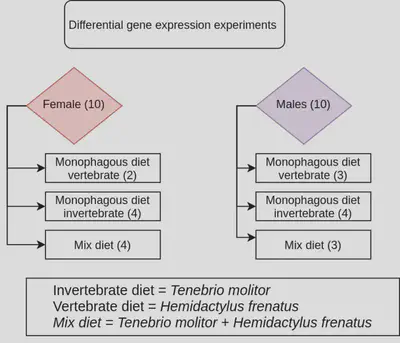
Later, you can plot your results and analyze them with packages like ggplot2 or bigpint; The data analyzed in this document correspond to an experiment designed to evaluate the differential expression of genes-transcribed in the venom glands of Phoneutria boliviensis, some individuals were subjected to the consumption of a strict invertebrate diet, others were subjected to a vertebrate diet and others a mix between vertebrates and invertebrates,also this experiment checked the differences between sexes.
Load required libraries
This time we are going to use some package from ~CRAN~ and others from ~Bioconductor~,
list_of_CRAN_packages <- c("tidyverse",
                           "magrittr",
                           "stringr",
                           "ggplot2",
                           "readr",
                           "ggrepel",
                           "ggpubr",
                           "pacman",
                           "BiocManager")

new_packages <- list_of_CRAN_packages[!(list_of_CRAN_packages %in% installed.packages()[,"Package"])]

if(length(new_packages)) install.packages(new_packages)

list_of_Bioconductor_packages <- c("BiocParallel",
                                   "DESeq2",
                                   "EDASeq",
                                   "edgeR",
                                   "bigPint")

new_packages <- list_of_Bioconductor_packages[!(list_of_Bioconductor_packages %in% installed.packages()[,"Package"])]

if(length(new_packages)) BiocManager::install(new_packages)
Once you have installed all this packages you can use pacman package to load them all at once.
pacman::p_load(c(list_of_Bioconductor_packages,list_of_CRAN_packages), install = F, character.only = T, update = F)
Before starting, the first thing we need is a file with the counts of each gene or transcripts, you can get this file from the BAM files with Rsubread with , or with HTSEQ with .
The file we are going to use here were obtained withHTSeq 0.13.5
, now, we are going to import it to
and the information about the experimental design.
Import count data
In this case our counts are in a .txt file delimited by tab, for this reason we are going to use read.delim().
CountData <-read.delim("~/Documentos/R/R_Transcriptome/Resultados DEG/DEGs_preliminareszip/HTSeqcount_EDITED_mapeo_clean_ALL_AraBAN.txt", sep = "\t")
head(CountData)
| Reference | HTSeqcount_mapeo_cleanAraBANFG2.bam.txt | HTSeqcount_mapeo_cleanAraBANFG4.bam.txt | HTSeqcount_mapeo_cleanAraBANFmix1.bam.txt | HTSeqcount_mapeo_cleanAraBANFmix2.bam.txt | HTSeqcount_mapeo_cleanAraBANFmix3.bam.txt | HTSeqcount_mapeo_cleanAraBANFmix4.bam.txt | HTSeqcount_mapeo_cleanAraBANFT1.bam.txt | HTSeqcount_mapeo_cleanAraBANFT2.bam.txt | HTSeqcount_mapeo_cleanAraBANFT3.bam.txt | HTSeqcount_mapeo_cleanAraBANFT4.bam.txt | HTSeqcount_mapeo_cleanAraBANMG2.bam.txt | HTSeqcount_mapeo_cleanAraBANMG3.bam.txt | HTSeqcount_mapeo_cleanAraBANMG4.bam.txt | HTSeqcount_mapeo_cleanAraBANMmix2.bam.txt | HTSeqcount_mapeo_cleanAraBANMmix3.bam.txt | HTSeqcount_mapeo_cleanAraBANMmix4.bam.txt | HTSeqcount_mapeo_cleanAraBANMT1.bam.txt | HTSeqcount_mapeo_cleanAraBANMT2.bam.txt | HTSeqcount_mapeo_cleanAraBANMT3.bam.txt | HTSeqcount_mapeo_cleanAraBANMT4.bam.txt |
|---|---|---|---|---|---|---|---|---|---|---|---|---|---|---|---|---|---|---|---|---|
| TRINITY_DN10022_c0_g1_i1 | 0 | 0 | 1 | 1 | 0 | 0 | 0 | 0 | 1 | 1 | 2 | 0 | 0 | 0 | 0 | 0 | 0 | 6 | 0 | 0 |
| TRINITY_DN10032_c0_g1_i1 | 6 | 14 | 123 | 9 | 18 | 11 | 2 | 15 | 21 | 13 | 11 | 6 | 14 | 3 | 14 | 22 | 2 | 1 | 2 | 2 |
| TRINITY_DN10055_c0_g1_i1 | 11 | 2 | 1 | 12 | 0 | 8 | 15 | 2 | 1 | 3 | 7 | 8 | 8 | 12 | 6 | 7 | 18 | 8 | 20 | 6 |
| TRINITY_DN10066_c0_g1_i1 | 2 | 1 | 3 | 7 | 0 | 6 | 0 | 3 | 13 | 11 | 3 | 7 | 9 | 11 | 1 | 4 | 2 | 4 | 7 | 1 |
| TRINITY_DN10100_c0_g1_i1 | 0 | 0 | 1 | 0 | 2 | 1 | 1 | 0 | 4 | 2 | 3 | 0 | 1 | 3 | 0 | 2 | 2 | 1 | 0 | 3 |
| TRINITY_DN10102_c0_g1_i1 | 1 | 9 | 30 | 12 | 0 | 12 | 5 | 25 | 43 | 16 | 22 | 15 | 21 | 33 | 13 | 8 | 21 | 20 | 14 | 9 |
We are going to shorten the column names because they are too long.
CountData_row_names <- CountData %>% dplyr::select(Reference)
base::row.names(CountData) <- CountData_row_names$Reference

CountData <-CountData[,-1]
colnames(CountData) %<>%
  str_remove(pattern = "HTSeqcount_mapeo_cleanAraBAN") %>%
  str_remove(pattern = ".bam.txt")
head(CountData)
| FG2 | FG4 | Fmix1 | Fmix2 | Fmix3 | Fmix4 | FT1 | FT2 | FT3 | FT4 | MG2 | MG3 | MG4 | Mmix2 | Mmix3 | Mmix4 | MT1 | MT2 | MT3 | MT4 |
|---|---|---|---|---|---|---|---|---|---|---|---|---|---|---|---|---|---|---|---|
| 0 | 0 | 1 | 1 | 0 | 0 | 0 | 0 | 1 | 1 | 2 | 0 | 0 | 0 | 0 | 0 | 0 | 6 | 0 | 0 |
| 6 | 14 | 123 | 9 | 18 | 11 | 2 | 15 | 21 | 13 | 11 | 6 | 14 | 3 | 14 | 22 | 2 | 1 | 2 | 2 |
| 11 | 2 | 1 | 12 | 0 | 8 | 15 | 2 | 1 | 3 | 7 | 8 | 8 | 12 | 6 | 7 | 18 | 8 | 20 | 6 |
| 2 | 1 | 3 | 7 | 0 | 6 | 0 | 3 | 13 | 11 | 3 | 7 | 9 | 11 | 1 | 4 | 2 | 4 | 7 | 1 |
| 0 | 0 | 1 | 0 | 2 | 1 | 1 | 0 | 4 | 2 | 3 | 0 | 1 | 3 | 0 | 2 | 2 | 1 | 0 | 3 |
| 1 | 9 | 30 | 12 | 0 | 12 | 5 | 25 | 43 | 16 | 22 | 15 | 21 | 33 | 13 | 8 | 21 | 20 | 14 | 9 |
And then you import a file with the information about the experimental design of your experiment, the first five column are the most important.
Coldata <- read.delim("~/Documentos/R/R_Transcriptome/Data/Samples_information.csv", sep = ",",stringsAsFactors = T)
head(Coldata)
| ID_Trinity | Grupo_intra | ID_sample | SEX | DIET | Number_sequences | N50 | GC. |
|---|---|---|---|---|---|---|---|
| AraBANFG2 | FG | FG2 | Female | Vertebrate | 33841 | 1259 | 36.7 |
| AraBANFG4 | FG | FG4 | Female | Vertebrate | 38790 | 1319 | 36.5 |
| AraBANFmix1 | Fmix | Fmix1 | Female | Mix | 64601 | 1545 | 35.2 |
| AraBANFmix2 | Fmix | Fmix2 | Female | Mix | 57329 | 1415 | 35.5 |
| AraBaNFmix3 | Fmix | Fmix3 | Female | Mix | 25620 | 932 | 36.1 |
| AraBANFmix4 | Fmix | Fmix4 | Female | Mix | 50688 | 1297 | 35.9 |
Differential gen expression with DESeq2
DESeqDataSetFromMatrix() function create a ~DESeqDataSet~ object to store the counts and the information about you experiment design in a single object, here you declare the comparisons you want to do, in this case we are going to compare de differential transcript expression between the sexes.
options(na.action = na.fail) #this option return an error if you NAs appears

dds_sex <- DESeqDataSetFromMatrix(countData=CountData,
                                  colData=Coldata,
                                  design =  ~ SEX)
## converting counts to integer mode
Optionally, you can delete the transcripts that do not fit certain number of counts, here we are going to ignore transcripts with less than 10 counts.
keep <- rowSums(counts(dds_sex)) >= 10 #prefiltrar un numero minimo de conteos
dds_sex <- dds_sex[keep,]
Also you can optimize the performance, precesing the number of cores that your computer are going to use to process the data with MulticoreParam() from BiocParallel.
register(MulticoreParam(7))
Then our ~DESeqDataSet~ object can be processed by DESeq() to find if there are differences between the sexes under a negative binomial model, you should read the offical documentation if you want more information.
Next, you can extract the results with results() function and store them in a dataframe.
dds_sex <- dds_sex %>%
        DESeq(., parallel = T)
## estimating size factors
## estimating dispersions
## gene-wise dispersion estimates: 7 workers
## mean-dispersion relationship
## final dispersion estimates, fitting model and testing: 7 workers
## -- replacing outliers and refitting for 313 genes
## -- DESeq argument 'minReplicatesForReplace' = 7
## -- original counts are preserved in counts(dds)
## estimating dispersions
## fitting model and testing
dds_sex_results <- dds_sex %>%
        results() %>%
        as.data.frame()
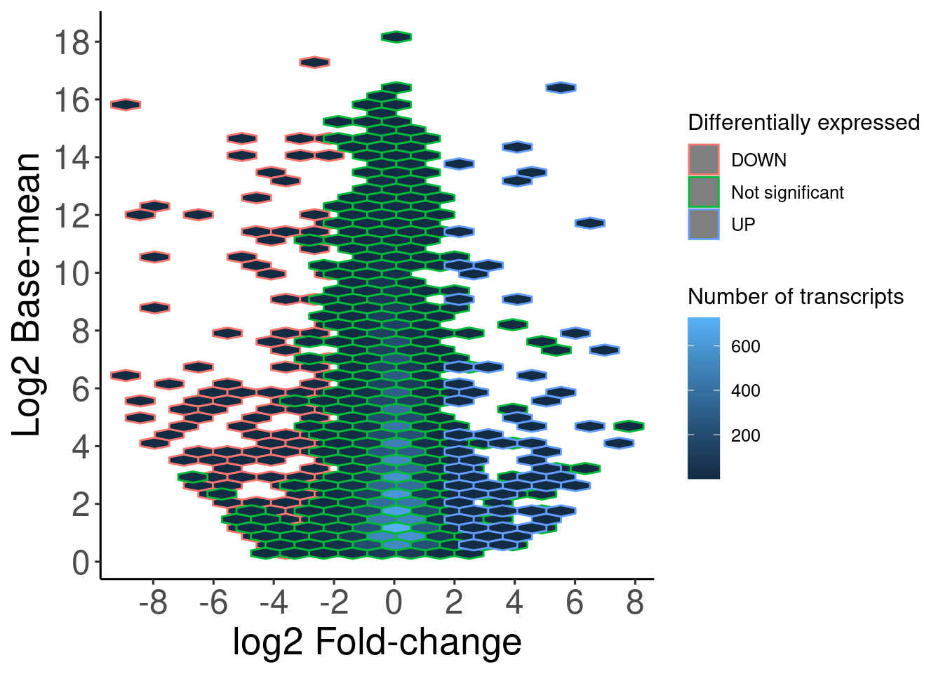
Now, you can add a new column to count the number of transcripts differentially expressed and set a threshold from -2 to +2 to the log2foldchange, take on mind this threshold is a log2, that means that if a transcript is found 4 times more in males than in the females it will have a log2Foldchange of 2.
dds_sex_results <- dds_sex_results %>%
        mutate(., differex =(case_when(log2FoldChange >= 2 & padj <= 0.05 ~ "UP",
                                       log2FoldChange <= -2 & padj <= 0.05 ~ "DOWN",
                                       log2FoldChange <= 2 | log2FoldChange >= 2 & padj >0.05 ~ "Not significant"))) %>% drop_na()
Finally you can filter the transcript differentially expressed and annotate them.
dds_sex_results %>%
        filter(., differex != "Not significant") %>%
        write.csv(., file = "~/Escritorio/DE_transcripts.csv", row.names = T)
Visualize the results
Multidimentional scaling (MDS)
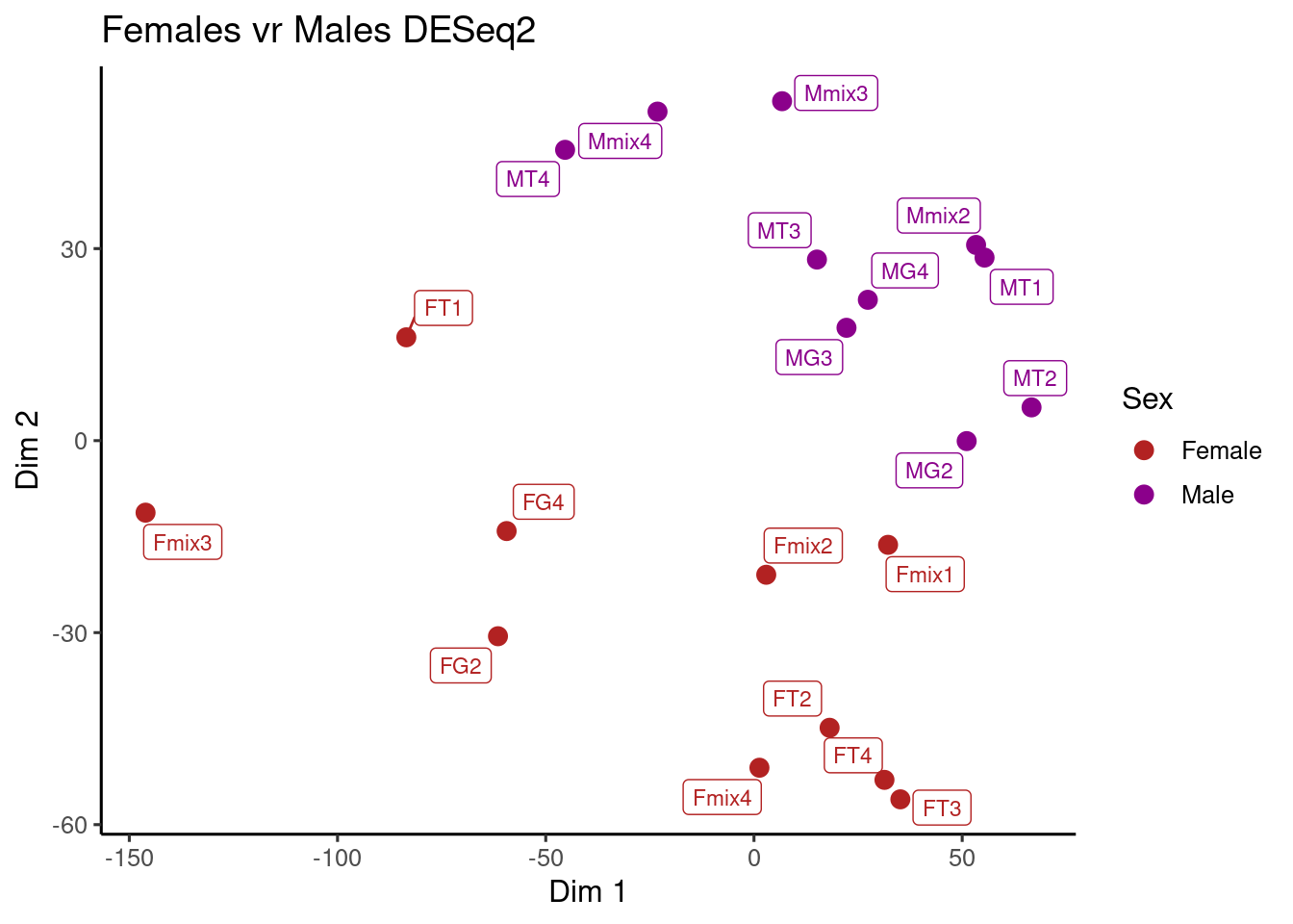
One technique in machine learning to visualize differences and create clusters is the MDS, base on the dissimilarity on a set of samples (distance), to create a MDS plot first we need to estimate the dispersion trend in or samples with vst(), then calc the distances with dist(), take the dissimilarities and represent them in a 2D space.
vsd_0 <- vst(dds_sex, blind = F) # calcualte dispersion trend
sampleDists <- dist(t(assay(vsd_0))) #Calculate distance matrix
sampleDistMatrix <- as.matrix( sampleDists ) # Create distance matrix
mdsData <- data.frame(cmdscale(sampleDistMatrix)) #perform MDS
mds <- cbind(mdsData, as.data.frame(colData(vsd_0)))
Now we can create a plot with ggplot2
F_vr_M_DESeq2_MDS <-  ggplot(mds, aes(X1,X2,color=SEX)) +
        geom_label_repel(aes(label = ID_sample), size = 3) +
        geom_point(size=3) +
        scale_color_manual(values =  c("#B22222","#8B008B"),
                           labels = c("Female", "Male"),
                           name = "Sex") +
        labs(title = "Females vr Males DESeq2",
             x = "Dim 1",
             y = "Dim 2") +
        theme_classic2()


F_vr_M_DESeq2_MDS
Volcano plot
Volcano plot is very useful to represent how many transcript are differentially expressed and how much, this plot basically shows the relation between log2 base-mean and the log2foldchange.
volcanoplot_phoneutria <- ggplot(data = dds_sex_results,
                                 aes(x = log2(baseMean),
                                     y = log2FoldChange, color = differex))+
        geom_hex(bins = 30) +
        labs(color = "Differentially expressed",
             fill = "Number of transcripts")+
  xlab("Log2 Base-mean")+ ylab("log2 Fold-change")+
        theme_classic2() +
  theme(axis.text.x = element_text(size = 18),
        axis.text.y = element_text(size = 18),
        axis.title.x = element_text(size = 20),
        axis.title.y = element_text(size = 20))+
        coord_fixed(ratio = 2/1) +
        scale_x_continuous(breaks = seq(from = 0, to = 20,2))+
        scale_y_continuous(breaks = seq(from = -10, to = 10,2)) +
        coord_flip()
## Coordinate system already present. Adding new coordinate system, which will replace the existing one.
volcanoplot_phoneutria
Parallel coordinates plot
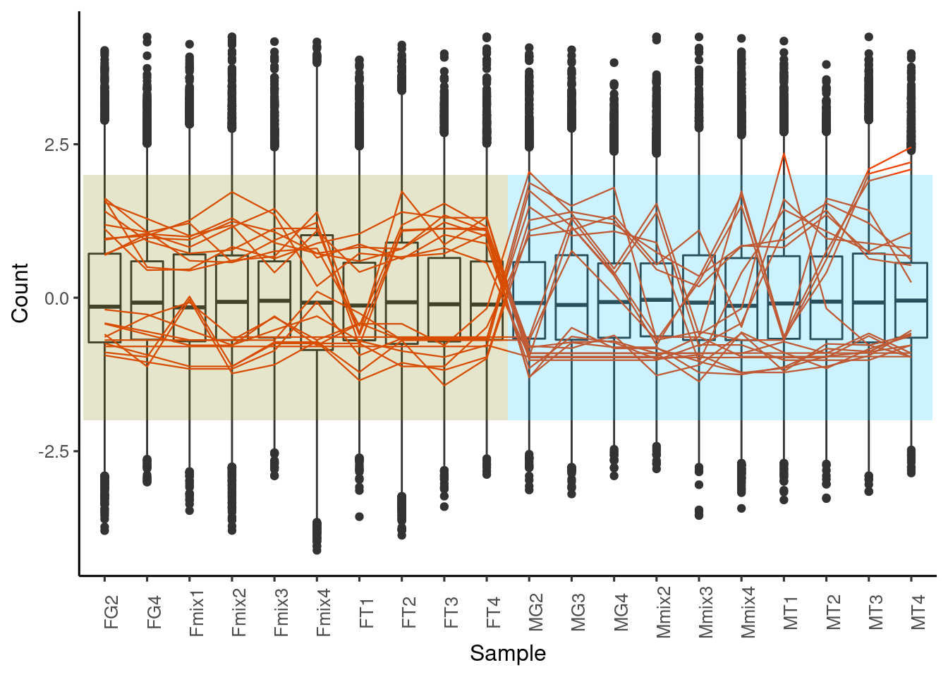
Other interesting plot it is the parallel coordinates plot, it can show you how some genes are differentially expressed along your samples or treatments, you can do it just with ggplot2 but bigPint makes the things easier.
Phoneutri_count_bigPint_SEX <- as.data.frame(dds_sex@assays@data$counts)
xlab <- colnames(Phoneutri_count_bigPint_SEX)
Phoneutri_count_bigPint_SEX$ID <- rownames(Phoneutri_count_bigPint_SEX)
Phoneutri_count_bigPint_SEX %<>%  dplyr::select(ID, everything())
rownames(Phoneutri_count_bigPint_SEX) <- NULL

#you have to change the column names for some shorten ones and separate the treatment and the samples by a point in order to work with bigPint
colnames(Phoneutri_count_bigPint_SEX) <- c("ID","F.1","F.2", "F.3", "F.4", "F.5","F.6", "F.7", "F.8", "F.9","F.10", "M.1", "M.2", "M.3",  "M.4", "M.5", "M.6", "M.7", "M.8",  "M.9","M.10")

head(Phoneutri_count_bigPint_SEX)
| ID | F.1 | F.2 | F.3 | F.4 | F.5 | F.6 | F.7 | F.8 | F.9 | F.10 | M.1 | M.2 | M.3 | M.4 | M.5 | M.6 | M.7 | M.8 | M.9 | M.10 |
|---|---|---|---|---|---|---|---|---|---|---|---|---|---|---|---|---|---|---|---|---|
| TRINITY_DN10022_c0_g1_i1 | 0 | 0 | 1 | 1 | 0 | 0 | 0 | 0 | 1 | 1 | 2 | 0 | 0 | 0 | 0 | 0 | 0 | 6 | 0 | 0 |
| TRINITY_DN10032_c0_g1_i1 | 6 | 14 | 123 | 9 | 18 | 11 | 2 | 15 | 21 | 13 | 11 | 6 | 14 | 3 | 14 | 22 | 2 | 1 | 2 | 2 |
| TRINITY_DN10055_c0_g1_i1 | 11 | 2 | 1 | 12 | 0 | 8 | 15 | 2 | 1 | 3 | 7 | 8 | 8 | 12 | 6 | 7 | 18 | 8 | 20 | 6 |
| TRINITY_DN10066_c0_g1_i1 | 2 | 1 | 3 | 7 | 0 | 6 | 0 | 3 | 13 | 11 | 3 | 7 | 9 | 11 | 1 | 4 | 2 | 4 | 7 | 1 |
| TRINITY_DN10100_c0_g1_i1 | 0 | 0 | 1 | 0 | 2 | 1 | 1 | 0 | 4 | 2 | 3 | 0 | 1 | 3 | 0 | 2 | 2 | 1 | 0 | 3 |
| TRINITY_DN10102_c0_g1_i1 | 1 | 9 | 30 | 12 | 0 | 12 | 5 | 25 | 43 | 16 | 22 | 15 | 21 | 33 | 13 | 8 | 21 | 20 | 14 | 9 |
datametrics_x <- dds_sex_results
datametrics_x$ID <- rownames(datametrics_x)

datametrics_x <- datametrics_x %>%
        select(ID, everything()) %>%  # create new column with the rownames
        select(., !differex)

rownames(datametrics_x) <- NULL # delete the rownames
datametrics_x <- list(F_M = datametrics_x) # create a list with the counts insida as a dataframe

datametrics_x$F_M <- as.data.frame(datametrics_x$F_M)
At the end your file should have this structure:
str(datametrics_x)
## List of 1
##  $ F_M:'data.frame':	17354 obs. of  7 variables:
##   ..$ ID            : chr [1:17354] "TRINITY_DN10032_c0_g1_i1" "TRINITY_DN10055_c0_g1_i1" "TRINITY_DN10066_c0_g1_i1" "TRINITY_DN10102_c0_g1_i1" ...
##   ..$ baseMean      : num [1:17354] 14.62 7.41 4.11 14.16 11.37 ...
##   ..$ log2FoldChange: num [1:17354] -1.5005 0.5838 -0.0362 0.1663 -0.652 ...
##   ..$ lfcSE         : num [1:17354] 0.594 0.504 0.525 0.371 0.413 ...
##   ..$ stat          : num [1:17354] -2.525 1.159 -0.069 0.448 -1.58 ...
##   ..$ pvalue        : num [1:17354] 0.0116 0.2466 0.945 0.6542 0.1141 ...
##   ..$ padj          : num [1:17354] 0.195 0.706 0.985 0.907 0.562 ...
Now you have to subset the genes you are interested for, in this case we are going to select the 20 most differently expressed genes.
tenSigGenes_phoneutria <- dds_sex_results %>% arrange(padj) %>%  filter(padj <= 0.05) %>% arrange(log2FoldChange)

tenSigGenes_phoneutria <- bind_rows(head(tenSigGenes_phoneutria,10),
                                    tail(tenSigGenes_phoneutria,10))
tenSigGenes_phoneutria$ID <- rownames(tenSigGenes_phoneutria)
rownames(tenSigGenes_phoneutria) <- NULL
tenSigGenes_phoneutria <- dplyr::select(tenSigGenes_phoneutria,"ID") %>% filter(row_number() <= 20)
tenSigGenes_phoneutria <- tenSigGenes_phoneutria[,1]
And then you create the plot step by step.
#prepare de data
dataID <- Phoneutri_count_bigPint_SEX$ID
data2 <- as.matrix(Phoneutri_count_bigPint_SEX[,-1])
d <- DGEList(counts = data2, lib.size = rep(1,20))
cpm.data.new <- cpm(d, TRUE, TRUE)
# Normalize de data
data2 <- betweenLaneNormalization(cpm.data.new, which="full", round=FALSE) %>% as.data.frame()

# Create matrix
data2$ID <- dataID
data2 = data2[,c(21,1:20)]
data2s = as.data.frame(t(apply(as.matrix(data2[,-1]), 1, scale)))
data2s$ID = as.character(data2$ID)
data2s = data2s[,c(21,1:20)]
colnames(data2s) <- colnames(data2)
nID = which(is.nan(data2s[,2]))
data2s[nID,2:length(data2s)] = 0

#Create plot
ret <- plotPCP(data = data2s, dataMetrics = datametrics_x, geneList = tenSigGenes_phoneutria, saveFile = FALSE, threshVar = "log2FoldChange", hover = F, lineSize = 0.4, lineColor = "orangered2")
colnames(data2s) <- c("Contin_Name", Coldata$ID_sample)

# extract and improve the plot
p <- ret[[1]]

p <-  p + theme_classic2() +
        scale_x_discrete(labels = dds_sex$ID_sample) +
        theme(axis.text.x = element_text(angle = 90)) +
        annotate("rect",
                 xmin = 0.5,
                 xmax = 10.5,
                 ymin = -2,
                 ymax = 2,
                 alpha = 0.2,
                 fill = "#808000") +
        annotate("rect",
                 xmin = 10.5,
                 xmax = 20.5,
                 ymin = -2,
                 ymax = 2,
                 alpha = 0.2,
                 fill = "#00BFFF")

p
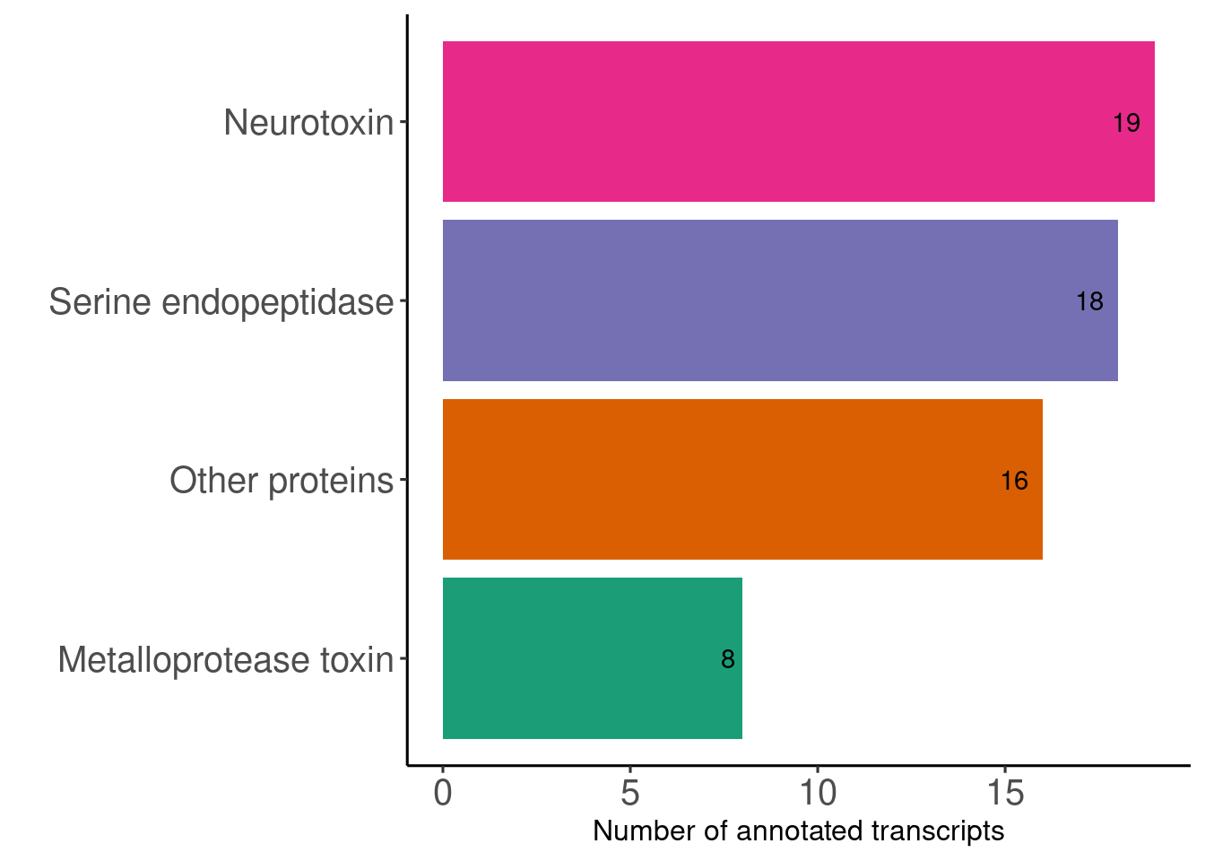
Summarize the number of genes
Once you have annotated your transcripts with tools like KEGG and GeneOntology, you can define categories and summarize you differential expressed an annotated genes with a barplot.
# load your differential expresed and annotated genes
summ <- read.csv("~/Documentos/R/R_Transcriptome/Data/Listas_DEG/filtered/ev_filtered_without_dup_for_cat.csv", header = T) %>%
        distinct(.,Contig_Name,.keep_all = T) %>%
        filter(.,New_cathegories != "Not related to venom")

# Add a filter
summ <- filter(summ, evalue <= 2.20e-30)

# Sort the categories
summ$New_cathegories <- factor(summ$New_cathegories, levels = names(sort(table(summ$New_cathegories),decreasing = F)))
summ %<>% group_by(.,New_cathegories) %>% dplyr::summarise(Cases =n())


# Create the final plot
p <- ggplot(summ) +
  geom_col(mapping = aes(x = New_cathegories,
                         Cases,
                         fill = New_cathegories))+
  geom_text(aes(x= New_cathegories,label= Cases,y = Cases),
              hjust = +1.5,
              position = position_dodge(.9))+
  coord_flip() +
  scale_fill_brewer(palette = "Dark2") +
  guides(fill = "none") +
  xlab(label = c(1:7)) +
  ylab("Number of annotated transcripts") +
  xlab("") +
  theme_classic2() +
  labs("")+
  theme(axis.text.y = element_text(size = 15),
        axis.text.x = element_text(size = 15))


p
Session info
## R version 4.1.3 (2022-03-10)
## Platform: x86_64-pc-linux-gnu (64-bit)
## Running under: Ubuntu 20.04.4 LTS
##
## Matrix products: default
## BLAS:   /usr/lib/x86_64-linux-gnu/blas/libblas.so.3.9.0
## LAPACK: /usr/lib/x86_64-linux-gnu/lapack/liblapack.so.3.9.0
##
## locale:
##  [1] LC_CTYPE=es_CO.UTF-8       LC_NUMERIC=C
##  [3] LC_TIME=es_CO.UTF-8        LC_COLLATE=es_CO.UTF-8
##  [5] LC_MONETARY=es_CO.UTF-8    LC_MESSAGES=es_CO.UTF-8
##  [7] LC_PAPER=es_CO.UTF-8       LC_NAME=C
##  [9] LC_ADDRESS=C               LC_TELEPHONE=C
## [11] LC_MEASUREMENT=es_CO.UTF-8 LC_IDENTIFICATION=C
##
## attached base packages:
## [1] parallel  stats4    stats     graphics  grDevices utils     datasets
## [8] methods   base
##
## other attached packages:
##  [1] huxtable_5.4.0              BiocManager_1.30.16
##  [3] pacman_0.5.1                ggpubr_0.4.0
##  [5] ggrepel_0.9.1               magrittr_2.0.3
##  [7] forcats_0.5.1               stringr_1.4.0
##  [9] dplyr_1.0.8                 purrr_0.3.4
## [11] readr_2.1.2                 tidyr_1.2.0
## [13] tibble_3.1.6                ggplot2_3.3.5
## [15] tidyverse_1.3.1             bigPint_1.8.0
## [17] edgeR_3.34.1                limma_3.48.3
## [19] EDASeq_2.26.1               ShortRead_1.50.0
## [21] GenomicAlignments_1.28.0    Rsamtools_2.8.0
## [23] Biostrings_2.60.2           XVector_0.32.0
## [25] DESeq2_1.32.0               SummarizedExperiment_1.22.0
## [27] Biobase_2.52.0              MatrixGenerics_1.4.3
## [29] matrixStats_0.62.0          GenomicRanges_1.44.0
## [31] GenomeInfoDb_1.28.4         IRanges_2.26.0
## [33] S4Vectors_0.30.2            BiocGenerics_0.38.0
## [35] BiocParallel_1.26.2
##
## loaded via a namespace (and not attached):
##   [1] utf8_1.2.2             shinydashboard_0.7.2   R.utils_2.11.0
##   [4] tidyselect_1.1.2       RSQLite_2.2.12         AnnotationDbi_1.54.1
##   [7] htmlwidgets_1.5.4      grid_4.1.3             munsell_0.5.0
##  [10] withr_2.5.0            colorspace_2.0-3       filelock_1.0.2
##  [13] highr_0.9              knitr_1.38             rstudioapi_0.13
##  [16] ggsignif_0.6.3         labeling_0.4.2         GenomeInfoDbData_1.2.6
##  [19] hwriter_1.3.2.1        bit64_4.0.5            farver_2.1.0
##  [22] vctrs_0.4.1            generics_0.1.2         xfun_0.30
##  [25] BiocFileCache_2.0.0    R6_2.5.1               locfit_1.5-9.5
##  [28] bitops_1.0-7           cachem_1.0.6           reshape_0.8.9
##  [31] DelayedArray_0.18.0    assertthat_0.2.1       promises_1.2.0.1
##  [34] BiocIO_1.2.0           shinycssloaders_1.0.0  scales_1.2.0
##  [37] nnet_7.3-17            gtable_0.3.0           rlang_1.0.2
##  [40] genefilter_1.74.1      splines_4.1.3          rtracklayer_1.52.1
##  [43] rstatix_0.7.0          lazyeval_0.2.2         hexbin_1.28.2
##  [46] broom_0.8.0            checkmate_2.1.0        yaml_2.3.5
##  [49] abind_1.4-5            modelr_0.1.8           GenomicFeatures_1.44.2
##  [52] backports_1.4.1        httpuv_1.6.5           Hmisc_4.7-0
##  [55] tools_4.1.3            bookdown_0.26          ellipsis_0.3.2
##  [58] jquerylib_0.1.4        RColorBrewer_1.1-3     Rcpp_1.0.8.3
##  [61] plyr_1.8.7             base64enc_0.1-3        progress_1.2.2
##  [64] zlibbioc_1.38.0        RCurl_1.98-1.6         prettyunits_1.1.1
##  [67] rpart_4.1.16           haven_2.5.0            cluster_2.1.3
##  [70] fs_1.5.2               data.table_1.14.2      blogdown_1.9
##  [73] reprex_2.0.1           aroma.light_3.22.0     hms_1.1.1
##  [76] mime_0.12              evaluate_0.15          xtable_1.8-4
##  [79] XML_3.99-0.9           jpeg_0.1-9             readxl_1.4.0
##  [82] gridExtra_2.3          compiler_4.1.3         biomaRt_2.48.3
##  [85] crayon_1.5.1           R.oo_1.24.0            htmltools_0.5.2
##  [88] later_1.3.0            tzdb_0.3.0             Formula_1.2-4
##  [91] geneplotter_1.70.0     lubridate_1.8.0        DBI_1.1.2
##  [94] dbplyr_2.1.1           rappdirs_0.3.3         Matrix_1.4-1
##  [97] car_3.0-12             cli_3.2.0              R.methodsS3_1.8.1
## [100] pkgconfig_2.0.3        foreign_0.8-82         plotly_4.10.0
## [103] xml2_1.3.3             annotate_1.70.0        bslib_0.3.1
## [106] rvest_1.0.2            digest_0.6.29          rmarkdown_2.13
## [109] cellranger_1.1.0       htmlTable_2.4.0        restfulr_0.0.13
## [112] curl_4.3.2             shiny_1.7.1            commonmark_1.8.0
## [115] rjson_0.2.21           lifecycle_1.0.1        jsonlite_1.8.0
## [118] carData_3.0-5          viridisLite_0.4.0      fansi_1.0.3
## [121] pillar_1.7.0           lattice_0.20-45        GGally_2.1.2
## [124] KEGGREST_1.32.0        fastmap_1.1.0          httr_1.4.2
## [127] survival_3.3-1         glue_1.6.2             png_0.1-7
## [130] bit_4.0.4              stringi_1.7.6          sass_0.4.1
## [133] blob_1.2.3             latticeExtra_0.6-29    memoise_2.0.1