Differential gene expression analysis with edgeR

edgeR is a popular package to the analysis of gene expression data from RNA sequencing technologies, it is useful to estimate the biological variation between replicate libraries, conduct tests of significance and it is an alternative to DESeq2 package, you can find a DESeq2 tutorial here and the edgeR’s official documentation here

Load required libraries

Firts, you have to load some ~CRAN~ and ~Biocondictor~ libraries to wragle the data, to make differential gene expression analyses and to create plots.

list_of_CRAN_packages <- c("tidyverse",
                           "magrittr",
                           "stringr",
                           "ggplot2",
                           "pacman",
                           "statmod",
                           "ggVennDiagram",
                           "BiocManager")

new_packages <- list_of_CRAN_packages[!(list_of_CRAN_packages %in% installed.packages()[,"Package"])]

if(length(new_packages)) install.packages(new_packages)

list_of_Bioconductor_packages <- c("edgeR",
                                   "BiocParallel")

new_packages <- list_of_Bioconductor_packages[!(list_of_Bioconductor_packages %in% installed.packages()[,"Package"])]

if(length(new_packages)) BiocManager::install(new_packages)

Once you have installed all this packages you can use pacman package to load them all at once.

pacman::p_load(c(list_of_Bioconductor_packages,list_of_CRAN_packages), install = F, character.only = T, update = F)

Import counts

You need to import the counts to , this counts can be obtained from BAM files with Rsubread package, or with with HT-SEQ.

Here, we going import the counts with read.delim() function, Also we are going to modify the columns and the column names with select() from dplyr (Tutorial here) and str_remmove() from stringr(Tutorial Here)

# Importar Coldata
CountData <-read.delim("~/Documentos/R/R_Transcriptome/Resultados DEG/DEGs_preliminareszip/HTSeqcount_EDITED_mapeo_clean_ALL_AraBAN.txt", sep = "\t")

# Set the "Reference" column as rownames
CountData_row_names <- CountData %>% dplyr::select(Reference)
base::row.names(CountData) <- CountData_row_names$Reference

#Rename the columns with a short and readable name

colnames(CountData) %<>% str_remove(pattern = "HTSeqcount_mapeo_cleanAraBAN") %>% str_remove(pattern = ".bam.txt")

CountData <-CountData %>%  select(.,!Reference)


# Importar information about the experimental design

Coldata <- read.delim("~/Documentos/R/R_Transcriptome/Data/Samples_information.csv", sep = ",", stringsAsFactors = T)

Differental gene expression with edgeR

Now you have to create an object to store the counts and the information about the experimental design with DGEList() function and filter counts under a minimum amount with filterByExpr().

y_sex <- DGEList(counts = CountData, 
                 group = Coldata$SEX)

keep <- filterByExpr(y_sex, min.count = 10)
y_sex <- y_sex[keep, , keep.lib.sizes=FALSE]

Then, your Coldata object that stores the information about your experimental design can be used to create a model matrix with model.matrix() function, this matrix will be used to estimate the dispertion among your samples with estimateDisp().

design <- model.matrix(~Coldata$SEX)
y_sex <- estimateDisp(y_sex, design, robust = T)

Now, with glmFit() and glmLRT() you can implement a generalized linear model

fit <- glmFit(y_sex, design)
edgeR_sex <- glmLRT(fit, coef = ncol(design))

Finally, you have to calculate the p.value adjusted or FDR and get the final result in a dataframe.

fdr <- p.adjust(edgeR_sex$table$PValue, "fdr") #Calculate the FDR using Benjamini & Hochberg test
edgeR_sex$table$FDR <- fdr 
colnames(edgeR_sex$table[5])<- "FDR"
edgeR_sex <- edgeR_sex$table #Get the final results

With this data you can use the same techniques to visualize the results in the same way you learnt with DESeq2package. https://diego-sierra-r.netlify.app/project/bioinformaticsdeseq2/.

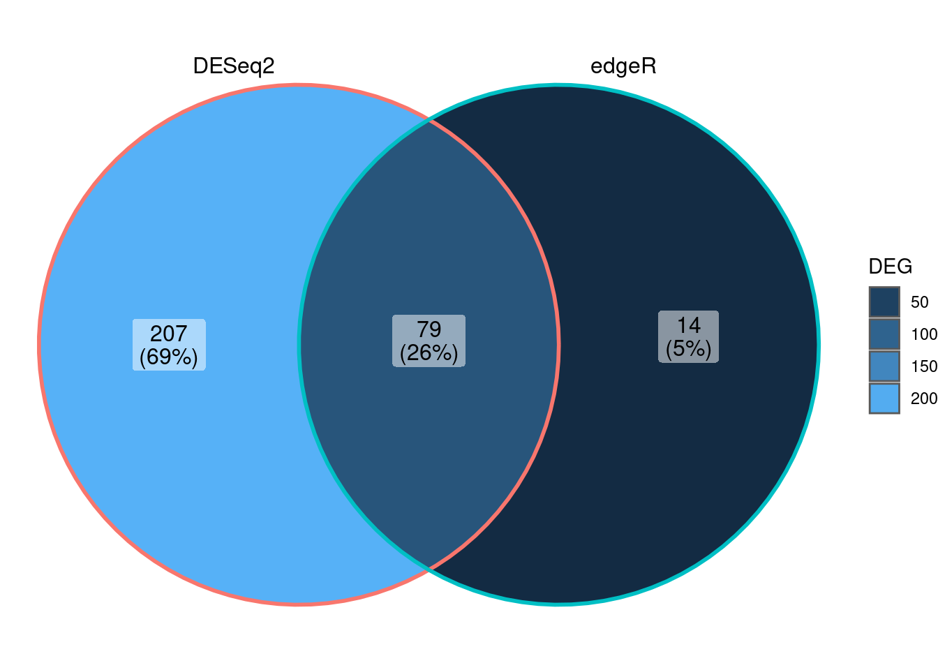
Also you can compare the results and the performance of both packages edgeR andDESeq2 with a venn diagram and other techniques.

#import DESeq2 results and filter the transcripts or genes differentially expressed
dds_sex_results <- read.csv("~/Documentos/R/R_personal_website_2.0/content/project/Bioinformatics:DESeq2/dds_sex_results.csv",row.names = 1) %>% 
        mutate(., differex =(case_when(log2FoldChange >= 2 & padj <= 0.05 ~ "UP",
                                       log2FoldChange <= -2 & padj <= 0.05 ~ "DOWN",
                                       log2FoldChange <= 2 | log2FoldChange >= 2 & padj >0.05 ~ "Not significant")))

#%>% drop_na() %>% filter(differex != "Not significant")

# Filter the differentially expressed transcripts or genes obtained with edgeR
edgeR_sex <- edgeR_sex %>% mutate(., differex =(case_when(logFC >= 2 & FDR <= 0.05 ~ "UP",
                                       logFC <= -2 & FDR <= 0.05 ~ "DOWN",
                                       logFC <= 2 | logFC >= 2 & FDR >0.05 ~ "Not significant"))) %>% drop_na() %>% filter(differex != "Not significant")

Finally you can create a Venn diagram with ggVennDieagram.

Venn_data <- list(DESeq2 = rownames(dds_sex_results),
                  edgeR = rownames(edgeR_sex))

ggVennDiagram::ggVennDiagram(Venn_data,)+
        guides(fill = guide_legend("DEG"))

Session info

## R version 4.1.3 (2022-03-10)
## Platform: x86_64-pc-linux-gnu (64-bit)
## Running under: Ubuntu 20.04.4 LTS
## 
## Matrix products: default
## BLAS:   /usr/lib/x86_64-linux-gnu/blas/libblas.so.3.9.0
## LAPACK: /usr/lib/x86_64-linux-gnu/lapack/liblapack.so.3.9.0
## 
## locale:
##  [1] LC_CTYPE=es_CO.UTF-8       LC_NUMERIC=C              
##  [3] LC_TIME=es_CO.UTF-8        LC_COLLATE=es_CO.UTF-8    
##  [5] LC_MONETARY=es_CO.UTF-8    LC_MESSAGES=es_CO.UTF-8   
##  [7] LC_PAPER=es_CO.UTF-8       LC_NAME=C                 
##  [9] LC_ADDRESS=C               LC_TELEPHONE=C            
## [11] LC_MEASUREMENT=es_CO.UTF-8 LC_IDENTIFICATION=C       
## 
## attached base packages:
## [1] stats     graphics  grDevices utils     datasets  methods   base     
## 
## other attached packages:
##  [1] BiocManager_1.30.16 ggVennDiagram_1.2.0 statmod_1.4.36     
##  [4] pacman_0.5.1        magrittr_2.0.2      forcats_0.5.1      
##  [7] stringr_1.4.0       dplyr_1.0.8         purrr_0.3.4        
## [10] readr_2.1.2         tidyr_1.2.0         tibble_3.1.6       
## [13] ggplot2_3.3.5       tidyverse_1.3.1     BiocParallel_1.26.2
## [16] edgeR_3.34.1        limma_3.48.3       
## 
## loaded via a namespace (and not attached):
##  [1] httr_1.4.2         sass_0.4.1         jsonlite_1.8.0     splines_4.1.3     
##  [5] modelr_0.1.8       bslib_0.3.1        assertthat_0.2.1   highr_0.9         
##  [9] cellranger_1.1.0   yaml_2.3.5         pillar_1.7.0       backports_1.4.1   
## [13] lattice_0.20-45    glue_1.6.2         digest_0.6.29      rvest_1.0.2       
## [17] RVenn_1.1.0        colorspace_2.0-3   htmltools_0.5.2    pkgconfig_2.0.3   
## [21] broom_0.7.12       haven_2.4.3        bookdown_0.25      scales_1.1.1      
## [25] tzdb_0.3.0         proxy_0.4-26       farver_2.1.0       generics_0.1.2    
## [29] ellipsis_0.3.2     withr_2.5.0        cli_3.2.0          crayon_1.5.1      
## [33] readxl_1.4.0       evaluate_0.15      fs_1.5.2           fansi_1.0.3       
## [37] class_7.3-20       xml2_1.3.3         blogdown_1.9       tools_4.1.3       
## [41] hms_1.1.1          lifecycle_1.0.1    munsell_0.5.0      reprex_2.0.1      
## [45] locfit_1.5-9.5     compiler_4.1.3     jquerylib_0.1.4    e1071_1.7-9       
## [49] rlang_1.0.2        units_0.8-0        classInt_0.4-3     grid_4.1.3        
## [53] rstudioapi_0.13    labeling_0.4.2     rmarkdown_2.13     gtable_0.3.0      
## [57] DBI_1.1.2          R6_2.5.1           lubridate_1.8.0    knitr_1.38        
## [61] fastmap_1.1.0      utf8_1.2.2         KernSmooth_2.23-20 stringi_1.7.6     
## [65] parallel_4.1.3     Rcpp_1.0.8.3       vctrs_0.3.8        sf_1.0-7          
## [69] dbplyr_2.1.1       tidyselect_1.1.2   xfun_0.30