Usually you have some sequences and you have to analyze them, you can do a lot of things with but first you have to import the sequences to , there are different alternatives and that depends on your purposes, this time we are going to work with seqinr package to make a variety of basic operations.

Reading a .fasta file

As always, first you have to load the libraries you will need.

library(seqinr)
library(tidyverse)

Then use read.fasta function with the path where is your file.

my_seqs <- read.fasta(file = "First50_neurotoxins.fasta")

my_seqs[1]

## $`pdb|1NTX|A`
##  [1] "r" "i" "c" "y" "n" "h" "q" "s" "t" "t" "r" "a" "t" "t" "k" "s" "c" "e" "e"
## [20] "n" "s" "c" "y" "k" "k" "y" "w" "r" "d" "h" "r" "g" "t" "i" "i" "e" "r" "g"
## [39] "c" "g" "c" "p" "k" "v" "k" "p" "g" "v" "g" "i" "h" "c" "c" "q" "s" "d" "k"
## [58] "c" "n" "y"
## attr(,"name")
## [1] "pdb|1NTX|A"
## attr(,"Annot")
## [1] ">pdb|1NTX|A Chain A, ALPHA-NEUROTOXIN"
## attr(,"class")
## [1] "SeqFastadna"

As you might notice, in this case each aminoacid is an element inside multiple strings, where each string is an aminoadic too, if you do not want this behavior you can use as.string argument collapse each sequence in a vector of a single element with all the aminoacids together.

my_seqs <- read.fasta(file ="First50_neurotoxins.fasta", as.string = T)

my_seqs[1]

## $`pdb|1NTX|A`
## [1] "ricynhqsttrattksceenscykkywrdhrgtiiergcgcpkvkpgvgihccqsdkcny"
## attr(,"name")
## [1] "pdb|1NTX|A"
## attr(,"Annot")
## [1] ">pdb|1NTX|A Chain A, ALPHA-NEUROTOXIN"
## attr(,"class")
## [1] "SeqFastadna"

Also you can detail how to interpret the sequences, for example if you want to precise that your .fasta file contains only proteins you can use the argument seqtype.

my_seqs <- read.fasta(file = "First50_neurotoxins.fasta", as.string = T, seqtype = "AA",forceDNAtolower = F)

my_seqs[1]

## $`pdb|1NTX|A`
## [1] "RICYNHQSTTRATTKSCEENSCYKKYWRDHRGTIIERGCGCPKVKPGVGIHCCQSDKCNY"
## attr(,"name")
## [1] "pdb|1NTX|A"
## attr(,"Annot")
## [1] ">pdb|1NTX|A Chain A, ALPHA-NEUROTOXIN"
## attr(,"class")
## [1] "SeqFastaAA"

Once you have imported your sequences you can make some analyzes or edit them, in the next example I’m going to delete the first codon in all the sequences, if you don’t understand the pattern used to match the first codon then you should go and review R tidiverse: stringr Part two (regular expressions) and regular expression cheatsheet

my_seqs <- my_seqs %>% map(.,~ str_remove(., pattern = "\\w{3}"))

my_seqs[1]

## $`pdb|1NTX|A`
## [1] "YNHQSTTRATTKSCEENSCYKKYWRDHRGTIIERGCGCPKVKPGVGIHCCQSDKCNY"

Basic operations

GC content

To find the the GC content of a sequence you can use GC() function or his variants (GC1(),GC2(),GC3()) if you are considering the lecture frame.

Take on mind that if you imported your sequences with the argument as.string equal to TRUE you have to split the your sequences and the use GC() function, but if you did not you can use GC() directly.

my_seqs$`pdb|1NTX|A` %>% 
        str_split(., pattern = "") %>% 
        unlist() %>% 
        GC()

## [1] 0.6666667

#Explore s2c() function, it makes the same but easier

Now we are going to do the same bat with all or sequences at same time with map function from purrr package.

my_seqs_GC <- my_seqs %>% map(.,~str_split(., pattern = "")) %>% map(.,unlist) %>% map(.,GC)

head(my_seqs_GC)

## $`pdb|1NTX|A`
## [1] 0.6666667
## 
## $`pdb|1DTK|A`
## [1] 0.7333333
## 
## $`pdb|1HOY|A`
## [1] 0.52
## 
## $NP_001350628.1
## [1] 0.4057971
## 
## $NP_001350625.1
## [1] 0.4179104
## 
## $`pdb|1D6B|A`
## [1] 0.7

Count the number of trinucleotides (codons)

If you are working with coding regions probably you are interested in knowing how many codons has your sequence, in this case count() function will help you.

my_DNA_seq <- "AGTGAGAGGAGGTAGAGCGAACGACGGAGCAACGATACGGACTGAGCATCGCCAAGTGAGAGGAGGTAGAGCGAACGACGGAGCAACGATACGGACTGAGCATCGCCAAGTGAGAGGAGGTAGAGCGAACGACGGAGCAACGATACGGACTGAGCATCGCCA" %>% s2c %>% str_to_lower %>% as.SeqFastadna
(counts <- seqinr::count(my_DNA_seq, wordsize = 3))

## 
## aaa aac aag aat aca acc acg act aga agc agg agt ata atc atg att caa cac cag cat 
##   0   6   2   0   0   0  12   3   6   9   6   3   3   3   0   0   5   0   0   3 
## cca ccc ccg cct cga cgc cgg cgt cta ctc ctg ctt gaa gac gag gat gca gcc gcg gct 
##   3   0   0   0   9   3   6   0   0   0   3   0   3   6  18   3   6   3   3   0 
## gga ggc ggg ggt gta gtc gtg gtt taa tac tag tat tca tcc tcg tct tga tgc tgg tgt 
##   9   0   0   3   3   0   3   0   0   3   3   0   0   0   3   0   6   0   0   0 
## tta ttc ttg ttt 
##   0   0   0   0

counts <- counts %>% as.data.frame()

Translate DNA to proteins

You can translate DNA to protein with translate() function, you can change the frame as you please.

my_protein <- my_DNA_seq %>% translate(frame = 1)
my_protein

##  [1] "V" "R" "G" "G" "R" "A" "N" "D" "G" "A" "T" "I" "R" "T" "E" "H" "R" "Q" "V"
## [20] "R" "G" "G" "R" "A" "N" "D" "G" "A" "T" "I" "R" "T" "E" "H" "R" "Q" "V" "R"
## [39] "G" "G" "R" "A" "N" "D" "G" "A" "T" "I" "R" "T" "E" "H" "R"

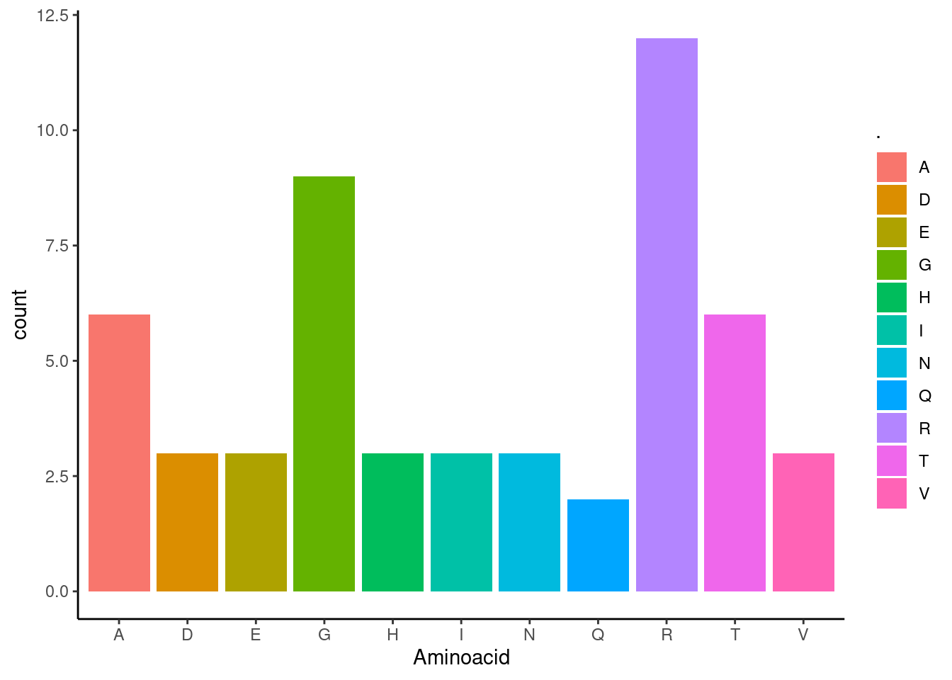
Then you can plot this sequence to find which amininoacids are more abundant.

my_protein <- my_protein %>% table() %>% as_data_frame() 

## Warning: `as_data_frame()` was deprecated in tibble 2.0.0.
## Please use `as_tibble()` instead.
## The signature and semantics have changed, see `?as_tibble`.
## This warning is displayed once every 8 hours.
## Call `lifecycle::last_lifecycle_warnings()` to see where this warning was generated.

ggplot(my_protein, aes(`.`,n, fill = `.`))+
  geom_col()+
  xlab("Aminoacid")+
  ylab("count")+
  theme_classic()

Reading alignments

You can read alignments with read.alignment(), this function can read different formats like FASTA, mase, clustal, msf and phylip, and then starting you analyzes.

path <- system.file("sequences/louse.fasta", package = "seqinr")
my_alignment <- read.alignment(path, format = "fasta")

Writing

Finally, after you make your analyses and modifications you can create a .fasta file with write.fasta() fasta.

write.fasta(file = path)