Epidemiological case: Logistic regression

Logistic Regression in Epidemiology
The idea of this project is to use logistic regression in an epidemiological context. Logistic regression is a very useful machine learning algorithm for classifying dichotomous variables (Alive/Dead, Sick/Healthy) and stands out for its speed and ease of interpretation compared to other methods.
In this guide we will review two cases, the first where logistic regression is not an effective tool to classify the development of Cardio Heart Disease according to multiple predictor variables and a second case where it is evaluated whether the thickness of a tumor can be related to whether a patient dies or not from cancer (melanome)
Before starting we will load the R packages that will be necessary to develop the guide.
## import
list.of.packages <- c("Epi", "janitor", "tidymodels", "glm2", "themis")
new.packages <- list.of.packages[!(list.of.packages %in% installed.packages()[, "Package"])]

if (length(new.packages))
  install.packages(new.packages)

library(Epi)
library(janitor)
library(tidymodels)
library(kableExtra)
library(glm2)
library(themis)
Cardio heart Disease case
For this case, we will use the ‘diet’ dataset from the ‘Epi’ package. We will select the variables that will be used as predictors and the cdh variable. We will standardize the variable names with the ‘clean_names()’ function and ee will modify the Cdh variable with ‘mutate()’, since logistic regression requires it to be a factor.
To learn more about the dataset we are using, you can type ‘?diet’ in the console.
## import
data(diet)
diet = diet |>
  select(energy,height,weight,fat,fibre,energy.grp,chd) |>
  clean_names("upper_camel") |>
  mutate(Chd = recode(Chd, `1` = "Yes", `0` = "No")) |>
  mutate(Chd = factor(Chd, levels = c("Yes", "No")))
Exploratory Data Analysis EDA
In the following two graphs we observe how there is a complete overlap in the relationship between weight and height of people who present CDH, this can indicate that despite there is a correlation between the variables weight and height, there is no clear distinction between the group of people who present CDH and those who do not.
The second graph shows us that there is also a complete overlap in weight between people who have CDH and those who do not, that is, the minimum and maximum weight limits of people who have CHD are both within the minimum and maximum limits of people who do not have CDH, this gives us an idea that at least the weight variable probably cannot be used to classify people who have CDH or not, you can try this exercise with the other variables.
## EDA
ggplot(diet, aes(Weight, Height, color = Chd)) + geom_point()## Warning: Removed 5 rows containing missing values or values outside the scale range
## (`geom_point()`).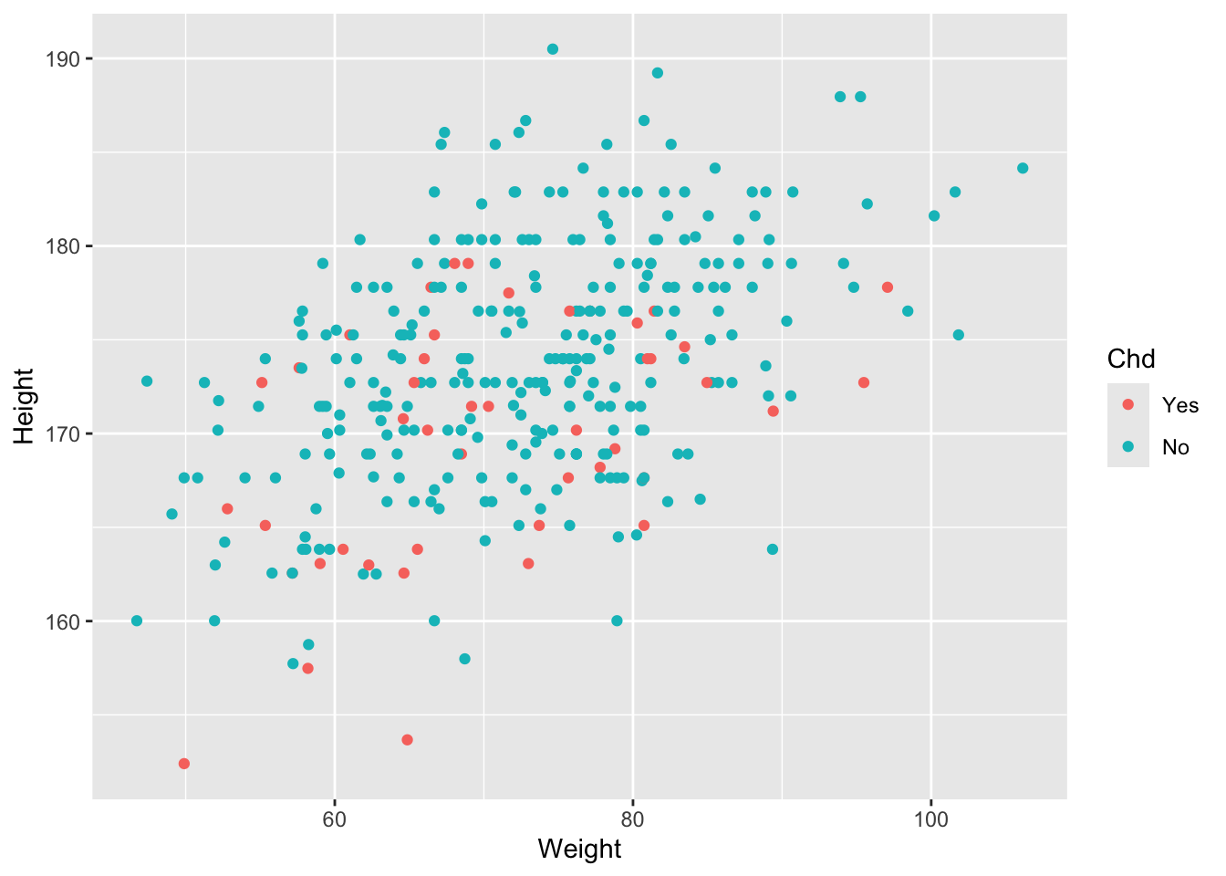
ggplot(diet, aes(Weight,Chd, color = Chd))+ geom_point()## Warning: Removed 4 rows containing missing values or values outside the scale range
## (`geom_point()`).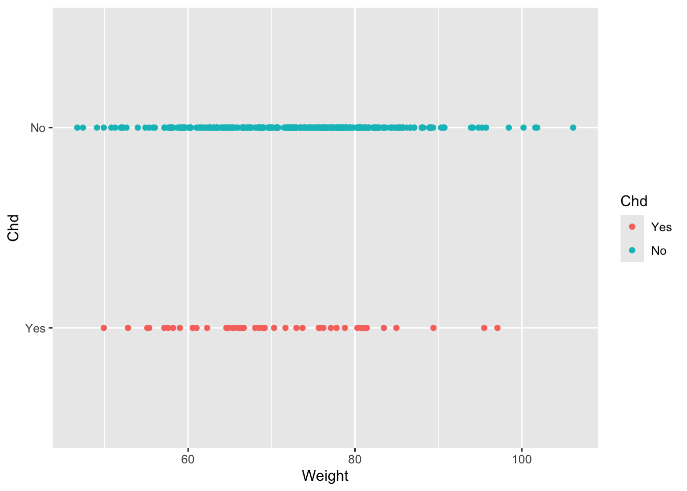
Creating the Logistic Regression Model
Despite what the exploratory analysis tells us, we will continue to perform logistic regression. To do this, we perform a 30/70 split of the original dataset to generate the data that will be used for training the model and for testing the model once generated.
## Splitting
set.seed(789)
Split3070 = initial_split(diet, prop = 0.7, strata = Chd)
DataTrain = training(Split3070)
DataTest = testing(Split3070)
head(DataTrain)## Energy Height Weight Fat Fibre EnergyGrp Chd
## 1 22.8601 181.610 88.17984 9.168 1.4000000 <=2750 KCals No
## 2 23.8841 165.989 58.74120 9.651 0.9350001 <=2750 KCals No
## 7 24.5261 179.070 81.19440 11.307 1.3210000 <=2750 KCals No
## 13 20.2325 173.990 61.46280 7.272 0.7110000 <=2750 KCals No
## 15 23.3816 166.370 66.45240 10.608 1.5350000 <=2750 KCals No
## 16 24.6795 158.750 58.24224 11.209 1.0030000 <=2750 KCals NoNow we will create the recipe that will contain all the information required to build the model, defining Chd as the variable to predict and all the other ‘( ~ .,)’ as predictor variables, we will also convert EnergyGrp into a dummy variable to facilitate interpretation and we will normalize the data with ‘step_normalize()’ via Z-score normalization.
## Recipe

RecipeDiet = recipe(Chd ~ ., data = DataTrain) |>
  step_dummy(EnergyGrp) |>
  step_normalize(all_predictors())
print(RecipeDiet)## ## ── Recipe ──────────────────────────────────────────────────────────────────────## ## ── Inputs## Number of variables by role## outcome: 1
## predictor: 6## ## ── Operations## • Dummy variables from: EnergyGrp## • Centering and scaling for: all_predictors()# Model Design
ModelDesignLogisticRegr = logistic_reg() |>
set_engine("glm") |>
set_mode("classification")Since we have defined the model, we will implement it with the traing dataset
# Building Fitting Workflow
WFModelDiet = workflow() |>
add_recipe(RecipeDiet) |>
add_model(ModelDesignLogisticRegr) |>
fit(DataTrain)con este modelo ajsutado, ahora podemos ver el valor de los coeficientes de cada una delas varaibles predictoras y el intercepto del modelo, el erros estarndar y especialmente el P.value de cada uno de ellos, estos nos infica que una variable esta aportando significativamente a la robustes del modelo de acuerdo aun treshold establecido, generalmente de 0.05 es este caso multiples variables tienves valores de p.value superiores como los son Energy, Fat and Fiber, then these variables are not contributing to improving the model.
This would not indicate that the model could be improved by eliminating such variables and that the present model would likely be deficient in trying to predict whether or not a person has CHD.
#print(WFModelDiet)
tidy(WFModelDiet)## # A tibble: 7 × 5
## term estimate std.error statistic p.value
## <chr> <dbl> <dbl> <dbl> <dbl>
## 1 (Intercept) 2.20 0.254 8.68 4.03e-18
## 2 Energy 0.194 0.515 0.375 7.07e- 1
## 3 Height 0.780 0.243 3.21 1.32e- 3
## 4 Weight -0.474 0.249 -1.90 5.70e- 2
## 5 Fat 0.287 0.397 0.723 4.70e- 1
## 6 Fibre 0.581 0.358 1.62 1.04e- 1
## 7 EnergyGrp_X.2750.KCals -0.309 0.342 -0.904 3.66e- 1Even so, for explanatory purposes we generate predictions, the ‘augment()’ function allows us to generate predictions in the set of data to be tested using predictions generated with the training dataset.
Now that we have the predictions we can use the ‘conf_mat()’ function to create a confusion matrix. This matrix, despite its name, simply allows us to see the relationship between correctly made predictions, false positives and false negatives.
According to the matrix, the model predicts well people who do not have CHD, but fails to completely classifying people who do have CHD.
# Prediction with augment()
DataTestWithPred = augment(WFModelDiet, new_data = DataTest)
conf_mat(DataTestWithPred, truth=Chd, estimate=.pred_class)## Truth
## Prediction Yes No
## Yes 0 2
## No 14 84Finally, we can use ‘FctMetricsSet()’ to check the accuracy, sensitivity and specificity of the model, below we can see how the sensitivity of the model is 0, since it cannot classify people who do present CHD.
FctMetricsSet = metric_set(accuracy, sensitivity, specificity)
FctMetricsSet(DataTestWithPred, truth = Chd, estimate = .pred_class)## # A tibble: 3 × 3
## .metric .estimator .estimate
## <chr> <chr> <dbl>
## 1 accuracy binary 0.84
## 2 sensitivity binary 0
## 3 specificity binary 0.977Melanoma case
This time we use the ‘melanome’ dataset for a case where the application of logistic regression is successful, and we correct a common problem in statistics which is unbalanced data, that is, one category presents many observations compared to another category and this makes it unfair (and incorrect) to make direct comparisons when applying machine learning models such as logistic regression.
Next, we’ll import the data we’ll use from the ‘boot’ package and filter it to keep only the data for people who died from melanoma and those who survived. To learn more about the dataset, you can use ‘?melanoma’ in the console.
## import
data(melanoma, package = "boot")
melanoma2 <- melanoma[melanoma$status != 3, c('status', "thickness")]
melanoma2$status[melanoma2$status == 2] <- 0
melanoma2 = melanoma2 |>
select(status, thickness) |>
mutate(status = recode(status, `1` = "Yes", `0` = "No")) |>
mutate(status = factor(status, levels = c("Yes", "No")))Now, as part of the exploratory analysis, we see that there is no complete overlap between the people who die from melanoma and those who do not. This suggests that logistic regression probably has more potential for success in this case. There are more specific and detailed methods to obtain this information, but this time we’ll keep it simple.
ggplot(melanoma2, aes(thickness,status, color = status))+ geom_point()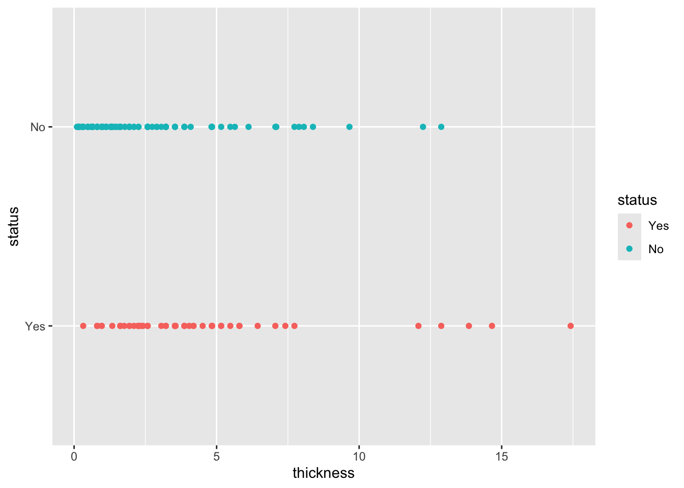
Before continuing, this time we will check if the data is balanced.
count(melanoma2, status) ## status n
## 1 Yes 57
## 2 No 134In the previous table we can see how the number of data we have of people who died from melanoma is much lower than the group of people who did not. We will solve this problem with the functions ‘step_downsample() / step_smote’, two popular methods to increase or decrease the number of observations in a dataset without affecting the distribution with respect to the original data.
## Splitting
set.seed(789)
Split3070 = initial_split(melanoma2, prop = 0.7, strata = status)
DataTrain = training(Split3070)
DataTest = testing(Split3070)
head(DataTrain)## status thickness
## 3 No 1.34
## 46 No 1.29
## 48 No 8.38
## 49 No 1.94
## 50 No 0.16
## 53 No 0.16## recipe
RecipeMela2 = recipe(status ~ thickness, data = DataTrain) |>
#step_normalize(all_predictors()) |>
step_downsample(status, under_ratio = 1) |>
step_smote(status, over_ratio = 1)
print(RecipeMela2)## ## ── Recipe ──────────────────────────────────────────────────────────────────────## ## ── Inputs## Number of variables by role## outcome: 1
## predictor: 1## ## ── Operations## • Down-sampling based on: status## • SMOTE based on: statusNow we build the model in a similar way as we did previously with the CHD case.
# Model Design
ModelDesignLogisticRegr = logistic_reg() |>
  set_engine("glm") |>
set_mode("classification")Now that our data is balanced and we have created the recipe and the model, we can adjust the training data, make predictions with the testing data, and review the confusion matrix.
# Building Fitting Workflow
WFModelMela = workflow() |>
  add_recipe(RecipeMela2) |>
  add_model(ModelDesignLogisticRegr) |>
  fit(DataTrain)
tidy(WFModelMela)
## # A tibble: 2 × 5
## term estimate std.error statistic p.value
## <chr> <dbl> <dbl> <dbl> <dbl>
## 1 (Intercept) 0.559 0.353 1.58 0.113
## 2 thickness -0.187 0.0938 -2.00 0.0459# Prediction with augment()
DataTestWithPred = augment(WFModelMela, new_data = DataTest)
conf_mat(DataTestWithPred, truth=status, estimate=.pred_class)## Truth
## Prediction Yes No
## Yes 13 11
## No 5 30This time, we find that the balanced logistic regression for this example contains proportionally fewer false negatives and false positives, and now the logistic regression better classifies people who died from melanoma.
Finally, we can review the metrics, this time the sensitivity is much better. Although this model is not perfect, it does provide information on how tumor thickness relates to the eventual death of a patient. This model would probably be much more robust if it included a larger number of observations to build the model.
FctMetricsSet = metric_set(accuracy, sensitivity, specificity)
FctMetricsSet(DataTestWithPred, truth = status, estimate = .pred_class)## # A tibble: 3 × 3
## .metric .estimator .estimate
## <chr> <chr> <dbl>
## 1 accuracy binary 0.729
## 2 sensitivity binary 0.722
## 3 specificity binary 0.732