Machine learning: Principal Component Analysis
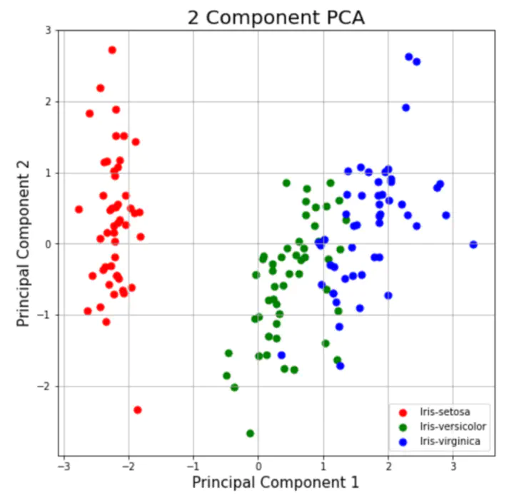
This document is a practical guide about ho to make a PCA, one of the most popular and spread techniques in unsupervised Machine learning used to visualize clusters and patterns in dataset with multiples variables.
We are going to use the iris dataset, it is as simple dataframe with four numerical variables and one categorical variable.
head(iris)## Sepal.Length Sepal.Width Petal.Length Petal.Width Species
## 1 5.1 3.5 1.4 0.2 setosa
## 2 4.9 3.0 1.4 0.2 setosa
## 3 4.7 3.2 1.3 0.2 setosa
## 4 4.6 3.1 1.5 0.2 setosa
## 5 5.0 3.6 1.4 0.2 setosa
## 6 5.4 3.9 1.7 0.4 setosaIf you want to work with your own data you have to import your file, https://diego-sierra-r.netlify.app/project/r-tidyversereadr/ about how to import files to {{< icon name=“r-project” pack=“fab” >}}
First, you have to load some required libraries:
library(factoextra) # to create the PCA## Loading required package: ggplot2## Welcome! Want to learn more? See two factoextra-related books at https://goo.gl/ve3WBalibrary(tidyverse) # To wrangle data## ── Attaching core tidyverse packages ──────────────────────── tidyverse 2.0.0 ──
## ✔ dplyr 1.1.4 ✔ readr 2.1.5
## ✔ forcats 1.0.0 ✔ stringr 1.5.1
## ✔ lubridate 1.9.4 ✔ tibble 3.2.1
## ✔ purrr 1.0.4 ✔ tidyr 1.3.1## ── Conflicts ────────────────────────────────────────── tidyverse_conflicts() ──
## ✖ dplyr::filter() masks stats::filter()
## ✖ dplyr::lag() masks stats::lag()
## ℹ Use the conflicted package (<http://conflicted.r-lib.org/>) to force all conflicts to become errorsPreparing the data
You can use numerical and categorical variables to create a PCA, but the true is there are other more appropriate techniques to cal the distances and represent categorical variables in the factorial space, for this reason we are going to use only numerical varibles to create the clusters with iris dataset.
clean_data <- select(iris, -Species) #delete categorical variableNow, with prcomp() we can create our PCA
PCA <- prcomp(clean_data)You can inspect and analyse some result summaries with summary(), for example, you can find how much variance are captured on each principal component looking the proportion of variance explained, the first PC has a 92.4%, and with PC2 they both together can captured the 97.7% of the variance, so you can discard the others PC without regrets.
summary(PCA)## Importance of components:
## PC1 PC2 PC3 PC4
## Standard deviation 2.0563 0.49262 0.2797 0.15439
## Proportion of Variance 0.9246 0.05307 0.0171 0.00521
## Cumulative Proportion 0.9246 0.97769 0.9948 1.00000Plotting our PCA
We are going to fviz_pca_ind() function from factoextra, to represent each observation on the multivariate space or “kendall’s shape space”
fviz_pca_ind(PCA) 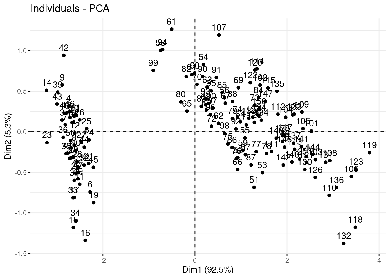
You can customize de PCA changing the geom argument and many others.
fviz_pca_ind(PCA, geom = "point")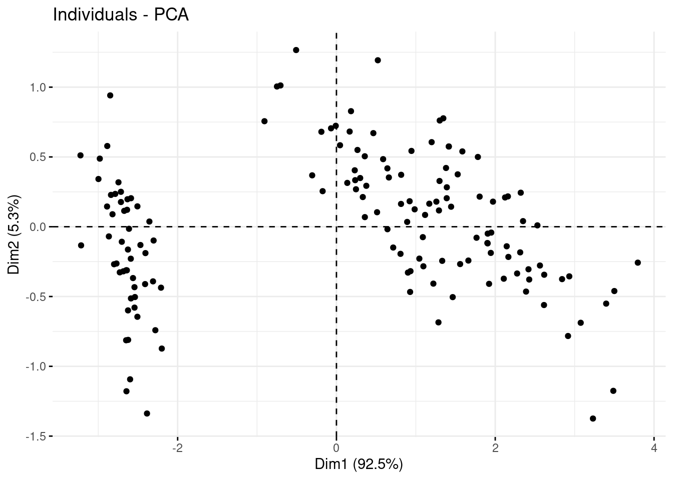
fviz_pca_ind(PCA, geom = "point", pointsize = 4, col.ind = "blue" )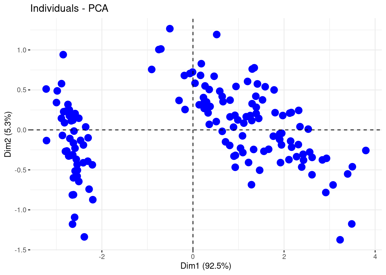
Or create guides
factoextra::fviz_pca_ind(PCA, label="none", habillage=iris$Species )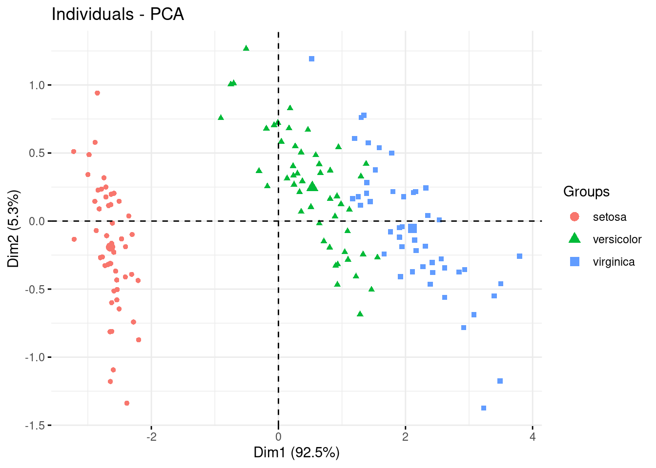
And finally you can add ellipses to your clusters
factoextra::fviz_pca_ind(PCA, label="none", habillage=iris$Species,
                                      addEllipses=TRUE, ellipse.level=0.95)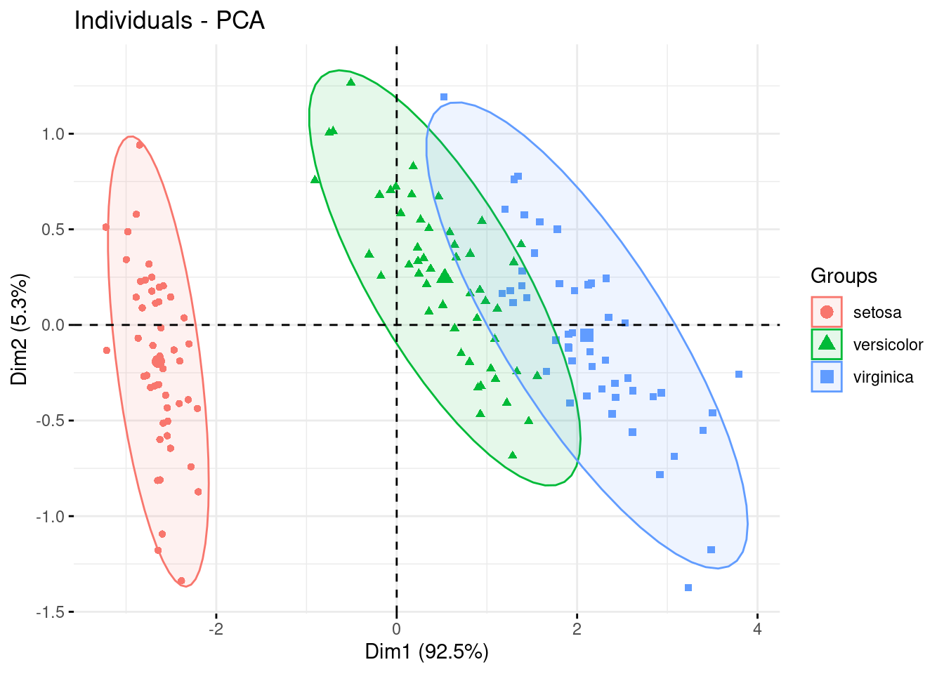
Take on mind this plot is a ggplot object so you can edit it even more using https://diego-sierra-r.netlify.app/project/r-tidiverseggplot2/