Machine learnig: Random forest for survival data

Random survival forest

A Random Survival Forest (RSF) is an ensemble machine learning method for analyzing right-censored survival data. It extends the idea of random forests to survival analysis on epidemiology, where the goal is to model the time until an event of interest occurs (e.g., death, relapse), and some observations might be censored (i.e., the event hasn’t happened by the end of observation).

In this guide, we will create a random survival forest to analyze how the mortality of a group may be related to a specific treatment in a group of patients followed over time to see the progression of their lung cancer. We will use the “veteran” dataset and the “randomForestSRC” package. This package must be installed directly from GitHub using the “devtools” package.

devtools::install_github("kogalur/randomForestSRC")

It is common that when handling epidemiological data we are faced with missing data, there are different techniques to address this problem and they generally involve data imputation, randomForestSRC has multiple input techniques, in this case we will do a quick imputation with the impute() function

#***************************************
# Imputation
library(randomForestSRC)
data(veteran, package = "randomForestSRC")

v.obj <- impute(
  status ~ .,
  veteran,
  ntree = 50,
  nimpute = 1,
  splitrule = "random"
)

We can create fast random forest, which is characterized by a lower number of iterations and greater computing performance. In this case, we will use the Random Forest algorithm to predict the final status of patients.

## grow a fast forest
obj <- rfsrc.fast(status ~ ., veteran)
print(obj)

##                          Sample size: 137
##                      Number of trees: 500
##            Forest terminal node size: 5
##        Average no. of terminal nodes: 7.928
## No. of variables tried at each split: 3
##               Total no. of variables: 7
##        Resampling used to grow trees: swor
##     Resample size used to grow trees: 87
##                             Analysis: RF-R
##                               Family: regr
##                       Splitting rule: mse *random*
##        Number of random split points: 10
##                      (OOB) R squared: -0.09177886
##    (OOB) Requested performance error: 0.06750372

When working with databases where there are many predictor variables, not all of them necessarily contribute or give robustness to the algorithm to classify or predict information, therefore it is important to review the number of variables that will ultimately be used in the model.

#Reducing number of variables for big data set

veteran2 <- impute(data = veteran, fast = TRUE)
xvar.used <- rfsrc(
  status ~ .,
  veteran2,
  ntree = 250,
  nodedepth = 4,
  var.used = "all.trees",
  mtry = Inf,
  nsplit = 100
)$var.used

xvar.keep  <- names(xvar.used)[xvar.used >= 1]
o <- rfsrc(status~., veteran2[, c("status", xvar.keep)])
print(o)

##                          Sample size: 137
##                      Number of trees: 500
##            Forest terminal node size: 5
##        Average no. of terminal nodes: 7.852
## No. of variables tried at each split: 3
##               Total no. of variables: 7
##        Resampling used to grow trees: swor
##     Resample size used to grow trees: 87
##                             Analysis: RF-R
##                               Family: regr
##                       Splitting rule: mse *random*
##        Number of random split points: 10
##                      (OOB) R squared: -0.07958758
##    (OOB) Requested performance error: 0.06674994

In this case, all variables are relevant to our random forest models.

An advantage of the randomForestSRC package is that it allows us to take survival time into account in epidemiological studies. We can specify this with the Surv() function and view partial effects with the partial() function.

#### Random survival forest

data(veteran, package = "randomForestSRC")
v.obj <- rfsrc(Surv(time,status)~., 
               veteran, 
               nsplit = 10, 
               ntree = 100)

partial.obj <- partial(v.obj,
       partial.type = "mort",
       partial.xvar = "age",
       partial.values = v.obj$xvar$age,
       partial.time = v.obj$time.interest)
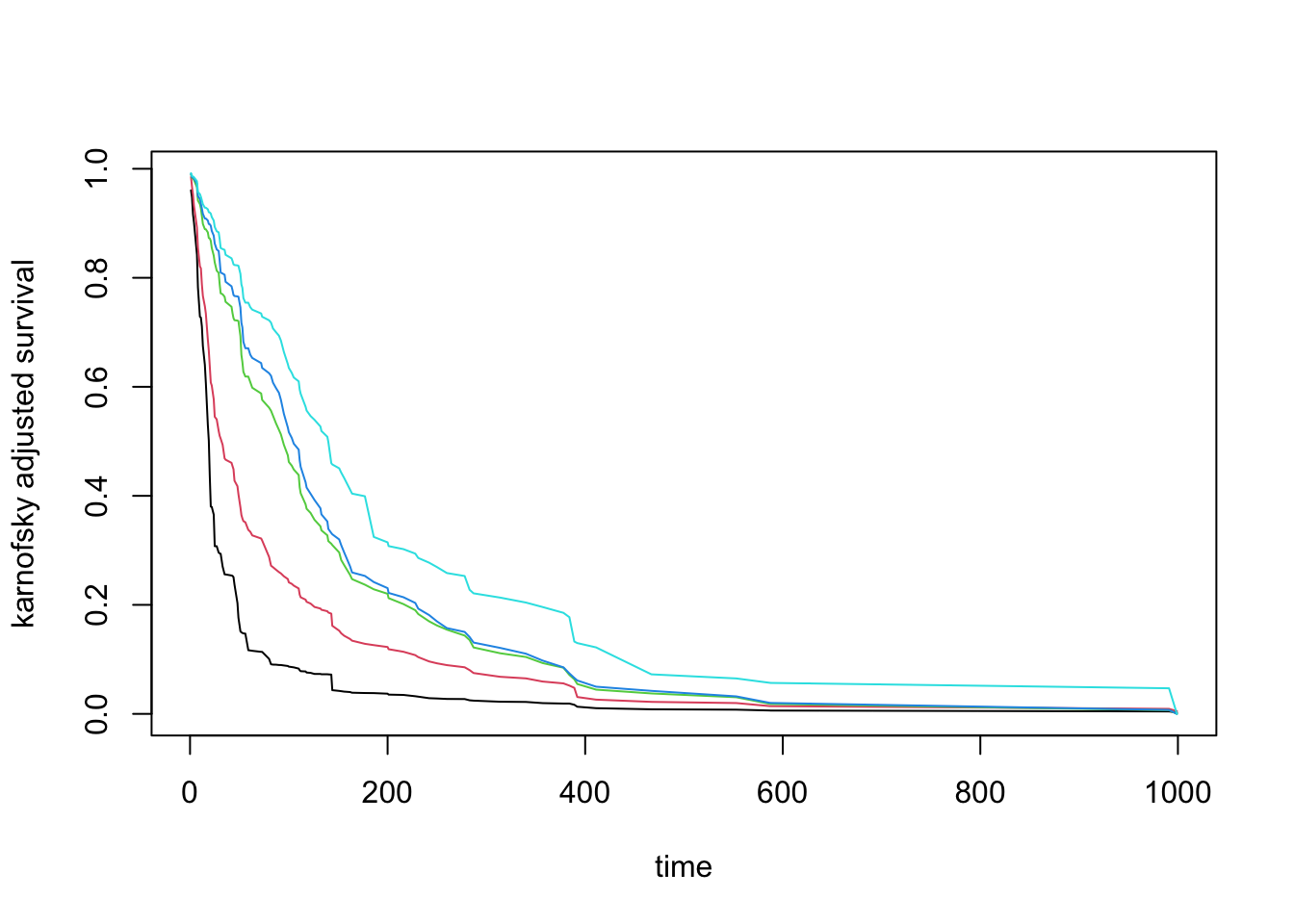
pdta <- get.partial.plot.data(partial.obj)

A very useful application when checking partial effects is to see the action of different variables in normality effects, for example seeing how the Karnofsky scale is associated with patient mortality.

karno <- quantile(v.obj$xvar$karno)
partial.obj <- partial(v.obj,
partial.type = "surv",
partial.xvar = "karno",
partial.values = karno,
partial.time = v.obj$time.interest)
pdta <- get.partial.plot.data(partial.obj)
matplot(
  pdta$partial.time,
  t(pdta$yhat),
  type = "l",
  lty = 1,
  xlab = "time",
  ylab = "karnofsky adjusted survival"
)